Ecosystems are inherently complex, and despite efforts to identify and model causal chains linking ecosystem disturbances with ecosystem response, there are inevitable discrepancies between observed and predicted conditions in the natural environment. Uncertainty, variability, and change all contribute to these differences, yet they are often ignored in predicting environmental problems. Statistical modeling techniques represent a general classification of tools that can help address discrepancies between predictions and observations, and Bayesian statistics in particular has recently been demonstrated to be a novel and effective tool for forecasting environmental pollutant problems because of its unique approach to quantifying uncertainty and variability.
Bayesian statistics
In 1763, an essay by Reverend Thomas Bayes, “Essay Towards Solving a Problem in the Doctrine of Chances,” was published in Philosophical Transactions of the Royal Society of London. More than 200 years later, the fundamental elements of this essay, including the introduction of a probabilistic relationship commonly referred to as Bayes' theorem (described in detail later in this article), form the foundation of Bayesian statistical analysis, a class of robust mathematical approaches to solving inverse probability problems.
Common strategies for statistical problem solving can be divided into three categories, each involving a different approach to quantifying the likelihood of an event relative to a set of all possible events. The first approach can be thought of as using a priori beliefs, which, in the case of a single roll of a six-sided die, might reflect an expectation that the die is fair, and therefore that the probability of each of the six possible outcomes (that is, 1, 2, … , 6) is exactly 1/6. A second approach is based on empirical evidence, in which our understanding of the underlying probability of events is based entirely on data. In the case of the six-sided die, this approach might involve rolling the die repeatedly and estimating the probability of each outcome as its observed relative frequency. In environmental problem solving, of course, this approach is often hindered by limited data and other complicating factors. Bayesian statistics, the third approach, provides a mechanism for combining a priori beliefs with potentially sparse empirical evidence to derive a posterior probability distribution. We describe this approach within the context of Bayes' theorem in the following section.
Bayes' theorem
Bayes' theorem can be written as Eq. (1),
where P(A) and P(B) represent the marginal probabilities of events A and B, respectively, while P(A|B) and P(B|A) represent the conditional probabilities of event A given that event B has occurred, and of event B given that event A has occurred, respectively. The probability P(A|B), in a Bayesian framework, is referred to as the posterior probability of event A, given that event B has occurred. In this context, Bayes' theorem states that the posterior probability of event A (that is, the probability of event A given that event B has occurred) is equal to the likelihood [written P(B|A)] times the prior probability distribution of event A [that is, P(A)], divided by the marginal distribution of event B. In this way, the prior probability distribution, the likelihood, and the posterior probability distribution provide the framework for and serve as the necessary elements of a Bayesian statistical problem.
Applications of Bayes' theorem
In more practical terms, Bayes' theorem allows scientists to combine a priori beliefs about the probability of an event (or an environmental condition, or another metric) with empirical (that is, observation-based) evidence, resulting in a new and more robust posterior probability distribution.
Understanding pollutant removal infrastructure performance
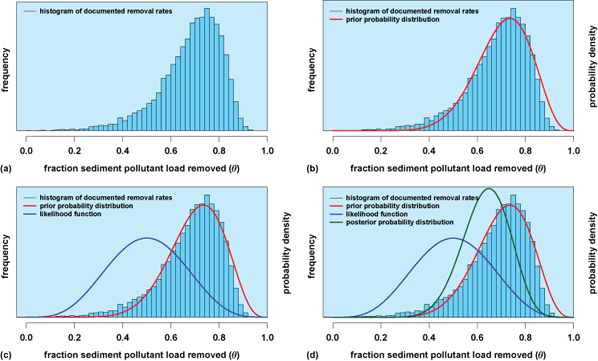
Figure 1 presents an example of how Bayes' theorem can be applied to solve environmental problems. In this hypothetical example, we are trying to improve our understanding of how effective stormwater management infrastructure systems are at removing sediment from stormwater runoff. While sediment often carries nutrients, metals, and other contaminants, sediment itself is also a pollutant in many environmental systems. In this problem, we represent the fraction of sediment removed by a stormwater management system as θ. Figure 1 presents the evolution of this understanding in a Bayesian framework, beginning with the development of a prior probability distribution. The prior probability distribution for θ is based on pollutant removal rate values in a published database documenting hundreds of studies, and is expressed in Fig. 1 first as a histogram of historic values (Fig. 1a), and then as a dashed line approximating the pollutant removal rate prior probability distribution (Fig. 1b). Hypothetical sediment removal rates from a new study site are then introduced through a likelihood function (solid line in Fig. 1 c), and finally the posterior probability distribution is calculated using Bayes' theorem (and represented by a dotted line in Fig. 1d).

Mathematically, Fig. 1 approximates the underlying histogram as a beta Be(θ|α, β) probability distribution with mean α/(α + β) and variance αβ/(α + β)2(α + β + 1), with parameters α and β set to 11 and 4.6, respectively. The likelihood is derived by modeling the hypothetical sediment removal rates from a new study site using a binomial probability distribution Bi(x|n, θ) with mean nθ and variance nθ(1 − θ), where x, in general, represents the number of positive outcomes out of n trials, and θ is the probability of a positive outcome in each trial. In this example, x represents the total mass of pollutant removed by the stormwater management infrastructure at a new study site, and n represents the total mass of pollutant entering the site. When expressed as a function of the unknown parameter θ, however, the likelihood [Eq. (2)] is a beta Be(θ|x + 1, n − x + 1) probability distribution with parameters n and x set to 8 and 4, respectively. Using Bayes' theorem, we combine the prior distribution and the likelihood to derive the posterior distribution for θ as follows in Eqs. (2) and (3),
where Eq. (3) is a beta Be(α′, β′) probability distribution with α′ = α + x and β′ = β + (n − x). Note that the right-hand side of Eq. (2) does not include a denominator, which we might expect based on Bayes' theorem [Eq. (1)], because it is simply a proportionality constant and does not affect our calculation of the posterior distribution. Put differently, once we recognize that Eq. (3) is a beta distribution, the values of α′ and β′ are the only information we need to formulate the posterior distribution for θ.
Predicting water quality conditions
Water quality is often measured by the concentration of one or more in situ pollutants (such as nutrients, bacteria, and organic compounds), and the suitability of a particular water body for its intended use (such as drinking water, recreation, or agricultural use) depends on whether or not the measured pollutant concentrations exceed water quality standard numeric limits. Because these pollutants often cannot be measured directly, scientists typically measure indicators that serve as potential surrogates for the pollutant of concern. The strength of the relationship between an indicator concentration and the concentration of the pollutant it supposedly represents varies widely depending on the type of pollutant. For example, in recreational and shellfish-harvesting waters throughout the United States, water quality is based on the concentration of nonpathogenic fecal indicator bacteria (FIB) such as fecal coliforms and Escherichia coli. These bacteria are used as a conservative indicator of fecal contamination and of the potential presence of harmful waterborne pathogens, which, while more directly linked to human and environmental health, are also much more difficult and costly to measure. Regardless of the specific pollutant and associated indicator, it is clear that not only the pollutant-indicator relationship, but also the spatial and temporal frequency of sampling and other factors might collectively contribute to uncertainty and variability in environmental condition forecasts. Here, we present a Bayesian approach to assessing water quality conditions using fecal coliform concentration measurements (reported in organisms per 100 ml) in a shellfish harvesting area as an example.
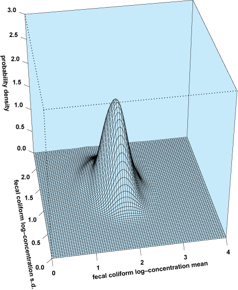
Like many other pollutants, FIB concentrations are commonly assumed to follow a lognormal LN (μ, σ) probability distribution with log-concentration mean (μ) and log-concentration standard deviation (σ). While this common probability model acknowledges natural spatial and temporal variability in FIB dispersion patterns, it (like other simple probability models) often fails to explicitly acknowledge other, more subtle sources of variability, including intrinsic sources arising from FIB concentration measurements and how FIB concentrations are calculated, all of which can lead not only to uncertainty in FIB concentration predictions, but to uncertainty in probability distribution parameters (that is, μ and σ) as well. In a Bayesian framework, we can explicitly acknowledge these uncertainties by first placing a prior probability distribution on the population parameters μ and σ (which may account for a priori beliefs about their potential values), then developing a likelihood function for μ and σ based on empirical evidence (in this case, using water quality samples), and, finally, deriving a joint posterior probability distribution for both. Results of this procedure are presented in Fig. 2, which includes a smoothed contour plot of the joint posterior probability density for the fecal coliform log-concentration mean (μ) and standard deviation (σ) for a sample site in eastern North Carolina.

Guiding environmental management decisions
Perhaps equally important as reflecting uncertainty in water quality predictions is understanding how that uncertainty might propagate into water quality–based management decisions. In a management context, the predicted conditions presented in Fig. 2 might be used to guide beliefs about the likelihood that future samples might indicate both a violation of the appropriate standards and a potential threat to human and environmental health. For example, water quality standards for shellfish-harvesting waters indicate it is unsafe to harvest shellfish when either the fecal coliform concentration median, geometric mean, or 90th percentile of a minimum of 30 water quality samples exceeds 14, 14, and 43 (all in organisms per 100 ml), respectively. When water quality sample concentrations exceed these numeric limits, the corresponding shellfish-harvesting area is closed, and signs are often posted warning the public of potential health risks (Fig. 3).

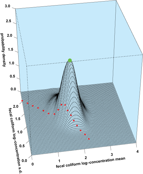
To better understand the uncertainty in fecal coliform concentration predictions, these numeric limits are translated into corresponding maximum allowable combinations of the fecal coliform log-concentration mean (μ) and log-concentration standard deviation (σ). These maximum allowable μ, σ pairs, when projected onto the three-dimensional joint (μ, σ) posterior probability space (dotted line in Fig. 4), provide an indication of how likely the water quality conditions are to yield a water quality sample in violation of the given standards. Put differently, we can imagine the dotted line in Fig. 4 “slicing off” a portion of the three-dimensional joint probability space to the bottom left of the figure, and the relative volume of this portion, sometimes called the confidence of compliance, can be thought of as the degree of confidence one can have that the water body will comply with water quality standards. In this example, the confidence of compliance is about 0.03 (or 3%).

To contrast the Bayesian-based confidence of compliance result with more common non-Bayesian strategies, a dot is plotted in Fig. 4, representing a potential point estimate of the most likely combination of μ and σ. A deterministic prediction of water quality conditions would probably be based solely on these point estimates, an approach that clearly ignores much of the potential variability in the future fecal coliform concentrations, and might lead to an oversimplified management assessment based not on a confidence of compliance, but on a simple statement of whether or not the water body violates the standard. In the case of the assessment results presented in Fig. 4, the deterministic approach would lead us to believe that future conditions will violate the given standard. A summary of monitoring assessment results for the station presented in Figs. 2 and 4, along with other neighboring water quality monitoring stations, is presented in the table. These results demonstrate how a Bayesian approach to predicting environmental conditions and to guiding management decisions provides a relatively robust approach to quantifying risk and protecting human and environmental health.
|
Station |
Bayesian assessment (confidence of compliance, %) |
Deterministic assessment (will standard be violated?) |
|---|---|---|
|
3 |
52 |
no |
|
4 |
44 |
yes |
|
7 |
<1 |
yes |
|
8 |
14 |
yes |
|
9 |
93 |
no |
|
25 |
3 |
yes |
|
28 |
96 |
no |
|
29 |
<1 |
yes |
|
35 |
80 |
no |
|
41 |
<1 |
yes |
|
84 |
13 |
yes |
[Disclaimer: The U.S. Environmental Protection Agency through the Office of Research and Development funded and managed some of the research described here. The present article has been subjected to the agency's administrative review and has been approved for publication.]
See also: Bayesian statistics; Environmental engineering; Environmental management; Water pollution


