The study of the shaking of the Earth's interior caused by natural or artificial sources. The revolution in understanding the Earth brought about by the paradigm of plate tectonics in the early 1960s provided a rationale that has since guided an intense period of investigation into the structure of the Earth's crust, mantle, and core. Plate tectonics provided Earth scientists with a kinematic theory for global tectonics that gave context to many of their studies. Ancient regions of crustal deformation could, for instance, be seen as the result of past plate boundary interactions, and the global distribution of earthquakes could be understood as the result of present plate interactions. The extraordinary insights into the nature of the solid Earth provided by kinematic plate tectonics also indicated new avenues in which to pursue basic questions concerning the dynamic processes shaping the Earth. Throughout the period in which plate tectonics was advanced and its basic tenets tested and confirmed, and into the latest phase of inquiry into basic processes, seismology (and particularly seismic imaging) has provided critical observational evidence upon which discoveries have been made and theory has been advanced. The use of the term image to describe the result of seismic investigations is closely linked mathematically to inversion and wavefield extrapolation and applies both to structures within the Earth and to the nature of seismic sources. See also: Plate tectonics
Theoretical seismology
A seismic source is an energy conversion process that over a short time (generally less than a minute and usually less than 1–10 s) transforms stored potential energy into elastic kinetic energy. This energy then propagates in the form of seismic waves through the Earth until it is converted into heat by internal (molecular) friction. Most earthquakes, for example, release stored elastic energy, nuclear and chemical explosions release the energy stored in nuclear and molecular bonds, and airguns release the pressure differential between a container of compressed air and surrounding water. Large sources, that is, sources that release large amounts of potential energy, can be detected worldwide. Earthquakes above Richter magnitude 5 and explosions above 50 kilotons or so are large enough to be observed globally before the seismic waves dissipate below modern levels of detection. The largest earthquakes, such as the 1960 event in Chile with an estimated magnitude of 9.6, cause the Earth to reverberate for months afterward until the energy falls below the observation threshold. Small charges of dynamite or small earthquakes are detectable at a distance of a few tens to a few hundreds of kilometers, depending on the type of rock between the explosion and the detector. The smallest of these may be detectable for only a few seconds. See also: Earthquake
Seismic vibrations are recorded by instruments known as seismometers that sense the change in the position of the ground (or water pressure) as seismic waves pass underneath. The record of ground motion as a function of time is a seismogram, which may be in either analog or digital form. Advances in computer technology have made analog recording virtually obsolete: most seismograms are recorded digitally, which makes quantitative analysis much more feasible.
Equation of motion
The dissipation of seismic energy in the Earth generally is small enough that the response of the Earth to a seismic disturbance can be approximated by the equation of motion for a disturbance in a perfectly elastic body. This equation holds regardless of the type of source, and is closely related to the acoustic-wave equation governing the propagation of sound in a fluid. Deviations of the elastic body away from equilibrium or rest are resisted by the internal strength of the body. An elastic material can be thought of as a collection of masses connected by springs, with the spring constants governing the response of the material to an externally applied force or stress. More formally, the strain or distortion of an elastic body when subjected to an applied stress is described with a constitutive relation, which is just a generalization of Hooke's law. Instead of just one spring constant, however, a generalized elastic solid needs 21 constants to completely specify its constitutive relation. Fortunately, the Earth is very nearly isotropic; that is, its response to an applied stress is independent of the direction of that stress. This reduces the complete specification of the constitutive relation from 21 to just 2 constants, the Lamé parameters λ and μ. A well-known result is that the equation of motion for an isotropic perfectly elastic solid separates into two equations describing the propagation of purely dilatational (volume changing, curl-free) and purely rotational (no volume changing, divergence-free) disturbances. These propagate with wave speeds α and β [Eqs. (1) and (2)],
 (1)
(1)respectively, where ρ is the density and the Lamé parameters have units of pressure (force/area).
Elastic-wave propagation
These velocities are also known as the compressional or primary (P) and shear or secondary (S) velocities, and the corresponding waves are called P and S waves. The compressional velocity is always faster than the shear velocity; in fact, it can be shown that mechanical stability requires that . In a fluid, μ = 0 and there are no shear waves. The wave equation then reduces to the common acoustic case, and the compressional wave is just the ordinary sound or pressure wave. In the Earth, α can range from a few hundred meters per second in unconsolidated sediments to more than 13.7 km/s (8.2 mi/s) just above the core–mantle boundary. (The fastest spot within the Earth is not its center, but just above the core–mantle boundary in the silicate mantle. The core, being predominantly iron, is in fact relatively slow.) Wave speed β ranges from zero in fluids (ocean, fluid outer core) to about 7.3 km/s (4.4 mi/s) at the core–mantle boundary. See also: Hooke's law; Special functions
A P wave has no curl and thus only causes the material to undergo a volume change with no other distortion. An S wave has no divergence, thus causing no volume change, but right angles embedded in the material are distorted. Explosions are relatively efficient generators of compressional disturbances, but earthquakes generate both compressional and shear waves. Compressional waves, by virtue of the mechanical stability condition, always arrive before shear waves.
Compressional and shear waves can exist in an elastic body irrespective of its boundaries. For this reason, seismic waves traveling with speed α or β are known as body waves. A third type of wave motion is produced if the elastic material is bounded by a free surface. The free-surface boundary conditions help trap energy near the surface, resulting in a boundary or surface wave. This in turn can be of two types. A Rayleigh wave combines both compressional and shear motion and requires only the presence of a boundary to exist. A Love wave is a pure-shear disturbance that can propagate only in the presence of a change in the elastic properties with depth from the free surface. Both are slower than body waves.
Solutions of the elastic-wave equation in which a wave function of a particular shape propagates with a particular speed are known as traveling waves. An important property of traveling waves is their causality; that is, the wave function has no amplitude before the first predicted arrival of energy. The complete seismic wavefield can be constructed by summing up every possible traveling wave, usually a countably infinite set. A traveling-wave formalism is useful especially when it is desirable to concentrate on particular arrivals of energy. An alternative set of solutions to the wave equation can be constructed by considering standing-wave functions. Individual standing waves by definition do not propagate, but rather oscillate throughout the body with a fixed spatial pattern. However, the sum of all possible standing waves must be equivalent to the sum of all possible traveling waves, because they must represent the same total wavefield. Standing waves, also known as free oscillations or normal modes, are useful representations of the wavefield in the frequency domain.
Ray theory
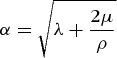
Traveling-wave or full-wave theory provides the basis for a very useful theoretical abstraction of elastic-wave propagation in terms of the more common notions of wavefronts and their outwardly directed normals, called rays (Fig. 1). The validity of the ray treatment can be deduced from full-wave theory by taking infinite frequency approximations that treat the seismic disturbances as pure impulses having essentially no time duration and unit amplitude. Ray theory makes the prediction of certain kinematic quantities such as ray path, travel time, and distance by a simple geometric exercise involving what is essentially a generalization of Snell's law. Ray theory can be developed in the context of an Earth comprising flat-lying layers of uniform velocities; this is a very useful approximation for most problems in crustal seismology and can be extended to spherical geometry for global studies. Expressions will be developed for travel time and distance in both geometries.
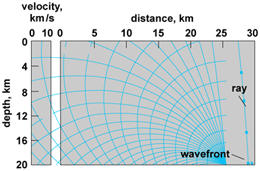
Figure 2 is a diagram showing the rays of a seismic wavefront in a single layer expanding away from a source, a single layer. It is apparent from this simple ray diagram that the rays will intersect the base of the layer and be reflected to the surface. Each ray leaves the source at an angle ι, known as the take-off angle or angle of incidence. This angle can be used to characterize each of the rays by Eq. (3),
where p is the ray parameter. This term characterizes uniquely each ray in a system of rays. Its physical meaning is very important; if the term slowness is used to describe the inverse of velocity, then p is the horizontal component of a ray's slowness. A vertical component q can also be defined, because unlike components of velocity the quantities p and q behave as vectors. This result makes it possible to cast the calculation of travel time and distance as geometric problems. Equation (4)
gives the time T(x) required to reach a given distance x from the source, and Eq. (5)
gives the distance reached by a ray of given ray parameter, X(p).
The first term on the right-hand side of Eq. (4) is the travel time of the vertical ray having a take-off angle of 0°, or p = 0. Equation (5) employs notation u to describe the slowness of the medium, rather than its velocity. Both Eqs. (4) and (5) are parametrized by layer thickness h and layer velocity α (or slowness u); and these are the unknowns needed to describe the Earth (α depends on the Lamé parameters and the density). Equation (4) is hyperbolic, which is sometimes observed in practice. This indicates that a simple representation of the Earth as a stack of uniform velocity layers might at times be reasonably close to reality.
Kinematic equations have been developed to describe what happens to rays as they impinge on the boundaries between layers. Figure 3a is a diagram of a single ray propagating in the stack of horizontal layers that define the model Earth. At each interface, part of the ray's energy is reflected, but a portion also passes through into the layer below. The transmitted portion of the ray is refracted; that is, it changes the angle at which it is propagating. The relationship between the incident angle and the refracted angle is exactly the same as that describing the refraction of light between two media of differing refractive index, as shown in Eq. (6).
This is the seismic analog of Snell's law. The left-hand side of Eq. (6) is the ray parameter for the ray in the upper layer, and the right-hand side is the ray parameter in the lower layer. Thus Snell's law for seismic energy is equivalent to stating that the ray parameter or the horizontal slowness is conserved on refraction. See also: Refraction of waves
Equation (7)
 (7)
(7)for multilayers describes the distance reached by a ray of given p after passing through n layers, each of which is associated with a slowness uk and thickness hk before being reflected to the surface. It is the sum of the individual contributions to X(p) from each of the layers. The equation for T(x) cannot be written as a simple sum of hyperbolic contributions, although doing so in some special situations can be a reasonable approximation to the real travel-time behavior. Because of this, complex seismograms are generally analyzed by using a “parametric” form such as
The generalization of these kinematic equations to the case where the medium slowness varies continuously with depth is straightforward. More care must be taken, however, in defining what happens to the ray at its deepest point of penetration into the medium. In Eq. (5), the ray is reflected from the base of the deepest layer. More generally, information is sought for the ray traveling downward, then reversing direction and traveling upward. In a medium with continuously varying velocities, this happens when the ray is instantaneously horizontal, that is, ι = 90° and the ray parameter or horizontal slowness p is equal to the medium slowness ; the term zmax is defined to be the turning point of the ray and is the deepest point in the medium sampled by the ray. The integral form of the distance equation is given by Eq. (8),
where represents any relationship of slowness versus depth.
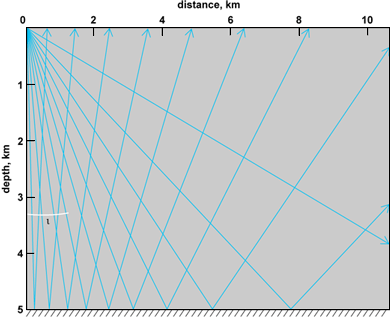
The case of a spherical Earth is treated by replacing the flat-Earth ray parameter by Eq. (9),
where r is the distance from the center of the Earth, v (r) is the velocity at that radius, and ι is the angle of intersection between the ray and the radius vector (Fig. 3b). The velocity function υ(r) denotes either α(r) or β(r), depending on the circumstance. The radius r0 at which ι = 90° is known as the turning radius of the ray and denotes the point at which the ray begins its journey back toward the surface. If υ(r) is a constant independent of radius, the ray path is straight but the turning point is still well defined. In a spherical Earth, the ray travels in the plane containing the source, the receiver, and the center of the Earth. Like its flat-Earth counterpart, the spherical-ray parameter must be conserved along the ray.
Seismogram synthesis
These simple geometric arguments can be extended to the computation of amplitudes provided that there are no sharp discontinuities in the velocity as a function of depth. More exact representations of the amplitudes and wave shapes that solve the full-wave equation to varying extents can be constructed with the aid of powerful computers; these methods are collectively known as seismogram synthesis, and the seismograms thus computed are known as synthetics. Synthetics can be computed for elastic or dissipative media that vary in one, two, or three dimensions.
The fundamental rationale for computing synthetics is rooted in the notion of the seismogram as an observable entity, and the distributions of Lamé parameters and density within the Earth as unknowns. In other words, it is the province of seismological imaging to estimate the three-dimensional variation of elasticity and density from observations of seismic-wave propagation. Beyond elucidation of basic structure, the variation of elasticity and density is a proxy for the variation of the chemical and thermal properties within the Earth. These in turn provide constraints on the long-term evolution of the Earth as a physical system.
Seismogram synthesis is an example of a forward problem; given a mathematical representation of the Earth and a model of the seismic source, attempts are made to compute synthetic seismograms (or some observables like travel time). For every forward problem, there is a concomitant inverse problem. The general statement of the inverse problem is: Given a set of observations of some measurable seismic disturbance at the Earth's surface, what can be said about that part of the Earth through which the disturbance passed and the characteristics of the source of the disturbance? The source and structural inverse problems are dichotomous in that something must be known about the source before the seismogram can be inverted for structure, and vice versa. This is not a problem in crustal or exploration imaging, where the properties of the artificial source are for the most part known and controlled. It is a problem when natural sources like earthquakes are used and specific steps must be taken either to isolate source and structure inversions or to do them jointly.
The development of inversion methods is a major area of research in seismology. The kinematic predictions of ray theory provide a useful starting point for a discussion of seismogram interpretation and inversion.
Crustal imaging
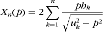
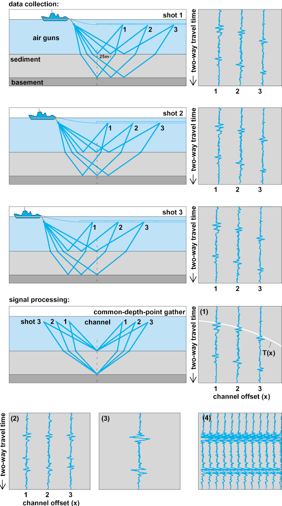
In a typical experiment for crustal imaging, a source of seismic energy is discharged on the surface, and instruments record the disturbance at numerous locations. Many different types of sources have been devised, from simple explosives to mechanical vibrators and devices known as airguns that discharge a “shot” of compressed air. The details of the source–receiver geometry vary with the type of experiment and its objective, but the work always involves collecting a large number of recordings at increasing distance from the source. Figure 4a shows a seismogram known as a T(x) resulting from one such experiment conducted at sea where an airgun source was fired and recordings were made by devices towed several meters below the sea surface from a research vessel. The strength of an arriving disturbance can be judged approximately by how dark the record appears.
This seismogram is complex, exhibiting a number of distinct arrivals with a variety of shapes and having amplitudes that change with distance, though they do not simply lose amplitude with increasing distance. Although this seismogram clearly does not resemble the structure of the Earth in any sensible way and is therefore not what would normally be thought of as an image, it can be analyzed to recover estimates of those physical properties of the Earth that govern seismic-wave propagation. Some simple deductions can be made by inspection. For instance, in a flat Earth the travel time equation is hyperbolic in distance. In the distance ranges up to about 15 km (9 mi), the observed T(x) seismogram in Fig. 4a indeed exhibits a number of segments which have a roughly hyperbolic shape. This can be taken immediately to indicate that the Earth here probably contains at least a few simple layers of uniform velocity. Some segments, particularly those developed at ranges greater than about 20 km (12 mi), do not show a hyperbolic form. In fact, their curvature is in the opposite sense to that expected for a hyperbolic reflection form. This indicates that the arrivals have propagated through a structure in which there is a continuous increase in velocity with depth, and are therefore turning or diving rays as discussed above.
The formal procedure of travel-time inversion involves deriving the turning-point depth for each ray parameter by using a formula for zmax that is obtained from Eq. (5) by an integral transform known as the Abel transform. This approach has been used extensively by seismologists, often very successfully. Methods have been developed that allow observational uncertainties to be included in the procedure so that the inversion calculates all of the possible υ(z) functions allowed by the data and their associated uncertainties, thereby giving an envelope within which the real Earth must lie. The approach has several difficulties principally associated with the nonlinear form of the X(p) equation. Although the desired quantity, υ(z), is single-valued (the Earth has only one value of velocity at any given depth), X(p) can be multivalued. X(p) also has singularities that are caused when the quantity under the square root goes to zero. Thus, care must be taken not to use rays that do not turn but are reflected at interfaces. In practice, separating out only those arrivals needed for the inversion can be very difficult. Furthermore, X(p) data are not actually observed but must be derived from observations. Methodologies that can overcome these problems attempt to linearize the equation with respect to small variations in X(p) and obtain an inversion that includes solution bounds derived from data uncertainties by linear programming.
Much of the difficulties have been further overcome by a coordinate transformation as shown in Eq. (10),
where τ(p) = T − pX.
The term τ(p) is known as the intercept time, and it can be thought of as the time that a vertically traveling ray takes to propagate upward from the turning point of a ray with ray parameter p. Although Eq. (10) still represents a nonlinear relationship between data τ(p) and desired Earth model u(z), the square root no longer presents a problem, and this leads to considerable stabilization of the inversion. The observed seismogram can be easily transformed to τ(p) by a process known as slant stacking, in which a computer search is made for all arrivals having a particular horizontal slowness; those data are summed; and using the appropriate X and T data, τ(p) is computed (Fig. 4b). Most importantly, like the desired α(z) function these τ(p) data are single-valued, so that deriving the υ(z) function amounts to a point-by-point mapping from τ(p) to α(z).
Much of this theory has been known for quite some time, but the τ(p) approach to inversion and analysis of seismic data did not see extensive application until relatively recently. One reason is that the quality and sparseness of many early seismic experimental data did not allow them to be treated with τ(p) methods. Data often comprised just a dozen or so seismograms obtained by using explosive charges and a few recording stations, the records from which were made in analog form usually on paper records. The example seismogram (Fig. 4a) is typical of modern marine seismic data in comprising several hundred equally spaced traces. The seismic source consisted of an array of airguns. Seismic arrivals are recorded on another vessel towing a hydrophone array more than 2 km (1.2 mi) long containing several thousand individual hydrophones. Recording on this ship is synchronized to the shooting on the other vessel. Ship-to-ship ranges are measured electronically and written onto the same system that records the seismic data together with other information such as shot times. This experimental method leads to the dense sampling of the seismic wavefield that is required for the correct computer transformation of the observed data into τ(p). The process is extremely demanding of computer time; it has come into common use only since relatively inexpensive, fast computers have made high computational power available to most researchers.
Figure 4c shows the result of analysis of the seismogram of Fig. 4a. It shows a profile of compressional-wave velocity against depth in the Earth at a location on the continental margin off East Greenland. The upper part of the crust where sedimentary layers are present is particularly complex, showing both uniform velocity layers, ones that show a gradational increase in velocity with depth, and one (at a depth of 3 km or 1.9 mi) in which the velocity is less than that of the layer above. This α(z) profile was constructed by the combination of several methodologies, including travel-time inversion from the τ(p) data in Fig. 4b and forward modeling of travel times and seismic amplitudes. Figure 4d depicts the rays that would propagate through such a structure; it is possible to recognize reflected arrivals that bounce off the interfaces between layers, and diving rays that smoothly turn in layers in which the velocity increases smoothly with depth.
Information from seismic waveforms
Real seismic disturbances have a finite time duration and a well-defined shape (see insert in Fig. 1). In passing through the Earth, any seismic disturbance changes shape in a variety of ways. The amount of energy reflected and transmitted at an interface depends on the ray incident angle (or equivalently on its ray parameter) and the ratio of physical properties across the boundary. It is sensitive both to the medium's compressional-wave and shear-wave velocities and to the ratio of densities. This is because, as well as splitting the arrival into reflected and refracted waves, boundaries act to convert waves from one mode of propagation to another. Thus, some of the compressional-wave energy incident on a boundary is always partitioned into shear energy.
Formulas for reflection and transmission coefficients are substantially more complex than those for the angles, and they are derived from considerations of traction across the boundary. At some incident angles the reflected energy becomes particularly strong. One point at which this happens is when the refracted wave travels horizontally below the interface, giving rise to a propagation mode known as a head wave, and essentially all the incident energy is reflected. This phenomenon is analogous to total internal reflection in optics. On the seismogram shown in Fig. 4a, there are several places where amplitudes become strong, and some can be related to critical-angle reflection, as this phenomenon is known in seismology.
Other strong regions correspond to places where energy is focused by the effect of changing subsurface gradients, which cause many diving rays to be returned to the surface near the same regions. Figure 4d was drawn by tracing a series of rays through the structure in Fig. 4c, with each ray incrementing in ray parameter by a fixed 0.005 s/km (0.008 s/mi). There are several regions where the density of rays returned to the surface is relatively sparse, while in other regions the density is very high (around 6 km or 3.7 mi, for instance). This pattern of amplitude variations can be used to refine models obtained by travel-time inversion and modeling to provide estimates of properties such as density, shear velocity, and attenuation (the amount of energy dissipated into heat by internal friction); however, it is often difficult to separate velocity and density uniquely, and estimates of acoustic impedance, the product of velocity and density, are more commonly derived.
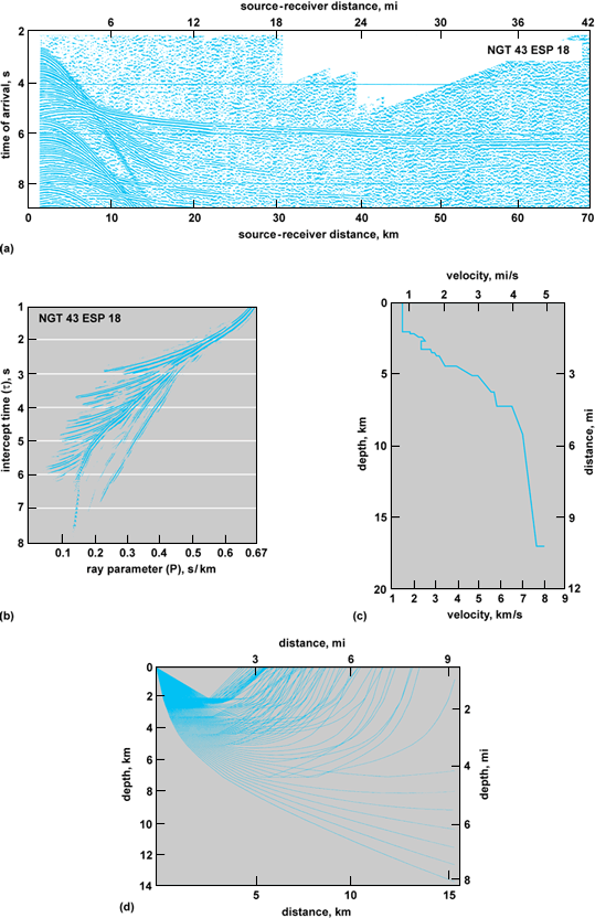
Waveform information can be employed either by forward modeling or by using the T(x) seismogram (Fig. 4a) directly in the inversion procedure. In the forward methodology a synthetic seismogram is calculated on a computer; a model structure, usually derived from travel-time inversion, is used as a starting point, and the effect of propagation of a real seismic source through the structure is computed. The synthetic is then compared to the observed data, misfits noted, and adjustments made to the model until a satisfactory fit is obtained (Fig. 5). Computation of synthetic seismograms is enormously consuming of computer time, and the various methods in use all apply some computational shortcuts that make the problem tractable. Like inversion of travel-time data from τ(p), the advent of modern computers has made the computation of synthetics more realistic, though only supercomputers allow this to be done routinely.
These very fast machines may also allow waveform data to be incorporated more directly into the inversion of seismic data. Clearly the desired aim is to make use of all the information that the entire seismogram contains to yield estimates of all the physical properties that contribute to the observed waveform of the seismogram. The problem is a highly nonlinear one, and can be regarded as an optimization problem often addressed with a nonlinear least-squares procedure in which computed and observed data are systematically compared and adjusted until a fit is obtained that satisfies some optimization criterion. The computational demands of such a procedure are such that the use of supercomputers is essential. The automatic inversion of the complete seismogram to recover all the physical property information that affects the seismic waveform is one of the most challenging areas of research in crustal seismology.
Two- and three-dimensional imaging
A volume of the crust can be directly imaged by seismic tomography. In crustal tomography, active sources are used (explosives on land, airguns at sea) so that the source location and shape are already known. Experiments can be constructed in which sources and receivers are distributed in such a way that many rays pass through a particular volume and the tomographic inversion can produce relatively high-resolution images of velocity perturbations in the crust (Fig. 6). Crustal tomography uses transmitted rays like those that pass from a surface source through the crust to receivers that are also on the same surface.
Because most applications of tomography make use of rays that are refracted in their passage through a structure, they provide representations of the crust expressed in terms of smoothly varying contours of velocity, or velocity anomaly with respect to some reference. Many interfaces within the crust are associated with relatively small perturbations in velocity and occur on relatively small spatial scales, making their imaging by tomographic techniques essentially impossible. The finely layered strata of a sedimentary basin, for instance, cannot be imaged by such an approach.
The most successful approach that has been devised to address the detailed imaging of crustal structure involves the use of reflected arrivals and is obtained by a profiling technique. In the reflection profile technique, energy sources and hydrophone (or geophone) arrays are the same as those used to create seismograms used for travel-time inversion; but in the profiling experiment, both are towed from the same vessel or moved along the ground together.
To produce an image from field recordings, they are first regrouped (gathered), corrected for the effect of varying source–receiver distance, and summed (stacked). The regrouping is made so that arrivals that are summed have come from the same reflection points and the time corrections are made assuming that all the arrivals obey hyperbolic travel times (see Fig. 7) and Eq. (4). Although the latter assumption is not completely correct, it is an acceptable approximation for the relatively small source–receiver offsets (the distance between the shot position and the receiver) used in this type of experiment. After summation, the resultant seismogram has very high signal-to-noise characteristics and appears as if it were obtained in an experiment in which source and receiver were fixed at zero separation and moved along the profile line. Such a record is shown in Fig. 8.
Mathematically, if a recording of the wavefield at the surface has been obtained, and since it is known that propagation obeys the wave equation, then the equation can be used to move the wavefield back to its point of origin; that is, it can be extrapolated back down into the Earth to the place where it began to propagate upward. Having done this, and applying some condition that allows the strength of the reflection to be determined, it becomes possible to recover an essentially undistorted image of the structure. A conceptual similarity to travel-time inversion can be recognized in this methodology. In travel-time inversion, formulas are used for X(p) or τ(p) to determine the turning-point depth of a ray. This could be restated by saying that the calculation extrapolates back down the ray from the surface to its turning point. Reflection imaging uses the wave equation to extrapolate the entire reflected wavefield back to its points of reflection, and can be considered the inversion methodology appropriate for the reflected wavefield.
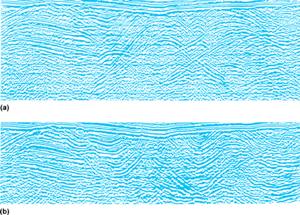
Several wavefield extrapolation methods have been developed, all of which involve several stages of manipulation of the data, and all are very demanding of computer time. Figure 8 shows one example in which data obtained in shallow water in a sedimentary basin showing complex deformation structures have been imaged to reveal a variety of geologically interpretable structures. The velocity field in the structure must be known very well (and may not be) for the imaging to be successful. Most extrapolation methods involve some form of approximation to the full-wave equation to make the computations tractable. Most, for instance, allow only mild lateral variations in velocity. To do the job in a complete sense requires use of the full-wave equation and operating on prestack data.
Advances, typically led by industry requirements, have seen surveys conducted to provide three-dimensional images, usually for petroleum reservoir evaluation. Survey lines are conducted on orthogonal grids in which the line spacing is as little as 50 m (160 ft) in both directions. Large exploration vessels carry two long hydrophone arrays set apart by 50 m (160 ft) on large booms or deployed on paravanes. Correct imaging of structure from such recordings requires a fully three-dimensional wavefield extrapolation procedure, and this has been developed successfully by using the power of supercomputers. Once the migrated image has been made, it can be manipulated in a smaller computer to observe structure in ways that cannot be achieved by conventional means. Horizontal slices can be made to show buried surfaces, diagonal cuts can be made to examine fault structure, and the whole image can be rotated to view the volume from any chosen direction.
The correct three-dimensional imaging of the Earth, either the whole Earth by tomographic means or crustal structure by tomography and reflection seismic imaging, represents a frontier research area in seismology. See also: Geophysical exploration; Group velocity; Phase velocity; Seismic exploration for oil and gas; Wave equation
Discoveries
Although the theory of plate tectonics allowed Earth scientists to recognize that the global mid-ocean ridge system represents the locus of formation of oceanic lithosphere, it gave little direct insight into the processes operating at these spreading centers. At a few scattered locations throughout the world, small slivers of oceanic crust known as ophiolites have been thrust into exposure onto continents as a result of collisional tectonics. Their study by geologists led to the proposition that large, shallow, relatively steady-state magma chambers are responsible for producing the crust at all but the slowest-spreading ridges. Efforts directed toward seismic imaging of spreading centers since 1980 produced some unexpected results. See also: Mid-Oceanic Ridge; Ophiolite
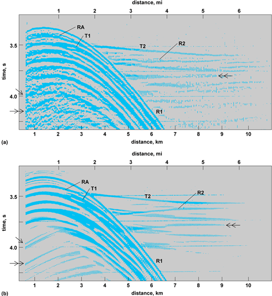
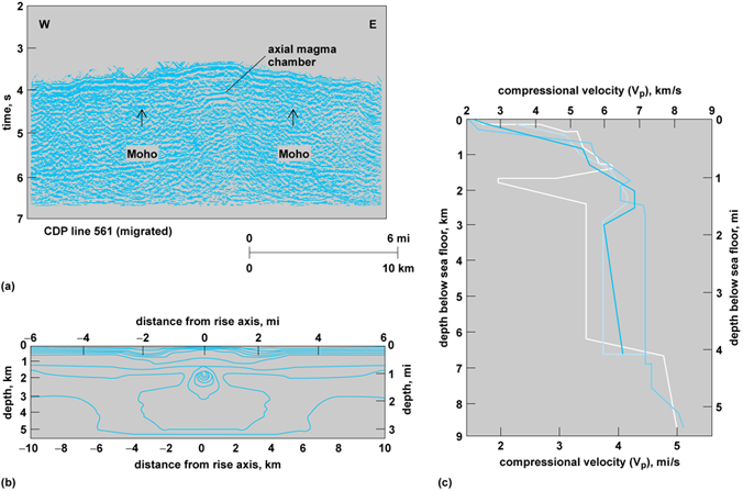
Reflection imaging of the fast-spreading center at the East Pacific Rise combined with two ship refraction seismic measurements in 1985, and later tomographic imaging, showed that a magma body indeed exists beneath the axis but that it is small and discontinuous (see Fig. 9). The magma body is so small, in fact, that the term chamber seems barely applicable. It is typically not more than 2–3 km (1.2–1.8 mi) wide, and the inferred region of melt (judged from the thickness of layers determined from the results of inversion and modeling of refraction seismic data) with greatly reduced velocities may be only a few hundred meters. This region is embedded in a broader zone of reduced velocities that may represent a region containing traces of melt but is more likely to be solid rock in which the temperature has been raised by proximity to the region of melt. The base of the crust, the Mohorovičić discontinuity (Moho), is a strong reflector formed very near the rise axis. See also: Moho (Mohorovičić discontinuity)
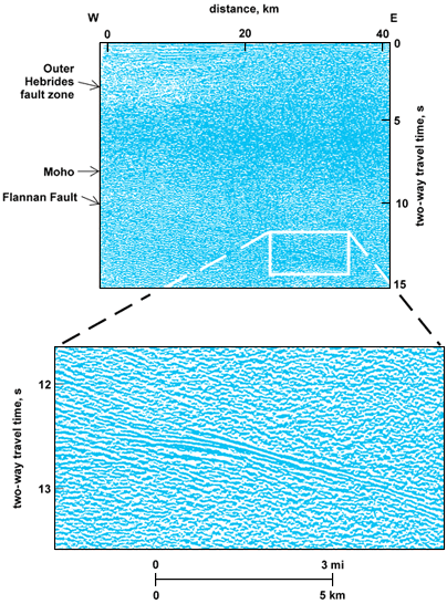
Images of continental crust and its underlying mantle have proven to be equally provocative (Fig. 10). Reflection profiling conducted on land in many regions of the world and on the shallow continental seas around Britain have shown that the deep crust is often characterized by an unreflective upper region and a band of strongly laminated reflections forming the lower third or so of the crust above a Moho that is quite variable in nature. The best available images show distinct events from within the mantle section itself. Mantle reflections may result from deep shear zones with reflectivity enhanced by deeply penetrating fluids. As exploration of the upper mantle has continued, it has become clear that structure in the mantle can be imaged by reflection methods to very great depths—perhaps even to the base of the lithosphere. It is possible that reflection methods will eventually be used to investigate the structure of the lithosphere as a whole, thereby complementing studies based on a different class of seismic methods that already have been developed. See also: Lithosphere
Global and regional seismograms
The basic unit of observation in global and regional seismology is a seismogram, but unlike their counterparts in crustal reflection and refraction, most seismometers used for larger-scale structural studies are geographically isolated from their neighbors. Thus the observational techniques and most methods of analysis used in global seismology have evolved quite differently from crustal seismology. Generally speaking, much more of each seismogram must be retained for analysis. This so-called spatial resolution gap is being closed slowly by the development of new portable instrumentation suitable for recording natural sources. Once these instruments are available in quantity, seismologists will be able to record seismic energy at closely spaced sites that will illuminate in much finer detail structures deep within the Earth.
Seismograms are classified according to the distance of the seismometer from the source epicenter. Those recorded within about 50–100 km (30–60 mi) of a large source are generally complex not only because of intervening structure but because the “dimensions” of the source are close to the propagation distance and different areas of stress release on the fault write essentially different seismograms. The term near-field is given to these seismograms to signify that the propagation distance for the seismic energy is less than a few source dimensions. Understandably, these seismograms are most useful for examining the details of the earthquake rupture. Beyond the near field to distances just past 1000 km (620 mi), the seismograms are dominated by energy propagating in the crust and uppermost mantle. These so-called regional seismograms are complicated, because the crust is an efficient propagator of high-frequency energy that is easily scattered; but there are still discernible arrivals. These seismograms are used to examine the velocity structure and other characteristics of relatively large blocks of crust. The domain beyond 1000 km (620 mi) is called teleseismic. Seismograms written at teleseismic distances are characterized by discrete and easily recognized body phases and surface-wave arrivals. These are relatively uncontaminated by crustal structure, and instead they are more sensitive to structure in the mantle and core.
Figure 11 shows both regional and teleseismic seismograms; since seismic-wave motion is vector motion, three components (up-down, north-south, and east-west) are needed to completely record the incoming wavefield. For the regional seismogram, the first arrival (Pg) is the direct P wave, which dives through the crust; the second arrival (Sg), beginning some 15 s after the Pg, is the crustal S phase. Even though explosions are inefficient generators of shear waves, it is common on regional seismograms to see substantial shear energy arising from near-source conversions of compressional to shear motion. The arrival time of the Pg phase can be picked easily, but the arrival time of Sg is somewhat more obscure. This is because some of the shear energy in the direct S is converted into compressional energy by scatterers in the crust near the receiver. This converted energy, traveling at compressional-wave speeds, must arrive before the direct S. The extended, very noisy wavetrains following the direct P and S are called codas; they represent energy scattered by small heterogeneities elsewhere in the crust. It is difficult to analyze these codas deterministically, and statistical procedures are often used. One result from the analysis of these and other seismograms is that the continental crust is strongly and three-dimensionally heterogeneous and scatters seismic energy very efficiently.
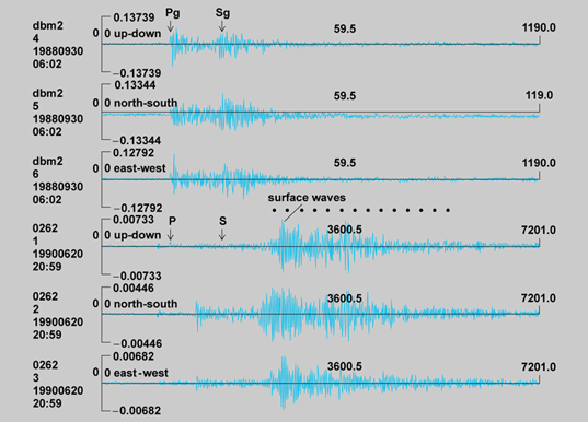
For the teleseismic seismogram, the teleseismic record is 60 times longer than the regional seismogram, and has been truncated only for plotting purposes. Plotted at this compressed time scale, it looks quite similar to the regional seismogram, but in fact there are important differences. The direct P and direct S waves are clearly evident; the S waves are larger on the horizontal components and larger than the P waves, a common feature for natural sources such as earthquakes. The very large-amplitude, long-period arrival starting some 20 min after the S are the surface waves. These waves are generally the most destructive in a major earthquake because of their large amplitude and extended duration. Between the direct P and the direct S are compressional body waves which have shallower take-off angles, and have bounced once (PP) or twice (PPP) from the surface before arriving at Palisades (the analogy here, though inverted, is like skipping a rock over water). The high level or energy between the S wave and the first surface wave is due to other multiply surface-reflected and -converted body waves, which are very sensitive to the structure of the upper mantle.
For purposes of analysis, the travel times of major phases have been inverted tomographically for large-scale structure. The International Seismological Centre (ISC) in England has been collecting arrival-time picks from station operators around the world since the turn of the century. Nearly one thousand stations report arrival-time picks consistently enough so that their accuracy can be judged without viewing the original seismograms. More than 2 million of these P-wave arrival times have been inverted tomographically for the structure of the lower mantle, the core, and the core–mantle boundary. These inversions show that the core–mantle boundary and the mantle just above it are very heterogeneous. Tomographic inversions of special P phases that transit the boundary show that the boundary may have topography as well. Estimates of the amplitude of this topography range from a few hundred meters to several kilometers, but further work must be done.
Direct P phases dive deeply into the mantle and are not very sensitive to upper mantle structure unless the earthquakes are within 25° or so of the seismometer. Multiple bounce body phases are more sensitive to upper-mantle structure, but these must be picked carefully from the teleseismic records. This has been done for several thousand seismograms situated in the United States and Europe, and the resulting models give very finely detailed views of the structure of the mid to upper mantle. These methods are sensitive enough to resolve the remnants of old subducted slabs in the lower mantle and the large keels of high-velocity material which seem to underlie most old continents.
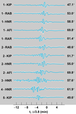
Going beyond tomographic methods requires analyzing more of the seismogram, for it is in the details of the wave shapes that information about major structures and the boundaries between them can be found. For example, surface waves disperse (different periods travel at different velocities) with wave speeds that depend on the fine details of the crust and upper mantle. An example of this dispersion can be seen in the Iranian seismogram (Fig. 11). Surface waves with longer periods arrive first and thus travel faster than surface waves at shorter periods. Measuring surface-wave dispersion is difficult but feasible, particularly for shallow earthquakes such as the Iranian event where the surface-wave arrivals dominate the seismogram. Seismologists began to measure dispersion in the late 1950s; some of the first applications of computers to seismological problems were the calculation of dispersion curves for oceanic and continental upper mantle and crust.
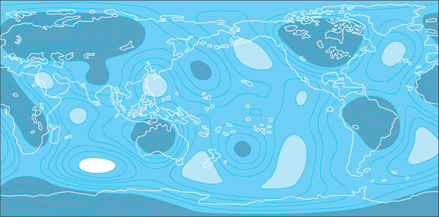
Measuring dispersion and other wave properties has evolved into a class of inversion procedures in which the entire seismogram is inverted directly for Earth structure. Such waveform inversion methods became feasible when computers became powerful enough to allow synthesis of most of the seismogram (see Fig. 12). After many years of operation, even the sparse global digital arrays collect enough data to contemplate tomographic inversions. The most successful of these experiments have combined the seismogram-matching techniques of waveform inversion with a generalization of the tomographic approach to obtain models of the three-dimensional variation of upper mantle structure. The vertical integration shown in Fig. 13 is a useful way of describing the geographic (two-dimensional) variation of a three-dimensional structure. Dark areas are fast relative to an average Earth, while light areas are slow. The darkest regions correspond to the oldest continental crust, known as cratons, while the lightest areas correspond to regions of active rifting either at mid-ocean ridges or at incipient oceans such as the Red Sea. See also: Waveform
Imaging the seismic source
The other half of the imaging problem in global seismology is constructing models of the seismic source. The simplest description of a so-called normal earthquake source requires two orthogonal force couples oriented in space. One force couple occurs on opposing sides of the rupture or fault surface and can be understood as the stress on either side of the fault induced by the earthquake rupture. The other couple is normal to the first and is required to conserve angular momentum. Implicit in this representation is the assumption that the earthquake is a point in both space and time (the point-source approximation), so that this type of source representation is known as a point-source double couple. Although there are some minor complications, the orientation of this double couple, and hence the orientation of the fault plane and the direction of rupture, can be inferred by analyzing the polarity of the very first P and S waves recorded worldwide. Thus this representation is known as a first-motion mechanism. It is not very difficult to make these observations provided that the instrument polarities are known, and the ensuing “beach-ball” diagrams are commonplace in the literature.
First-motion representations of seismic sources are the result of measurements made on the very first P waves or S waves arriving at an instrument; therefore they represent the very beginning of the rupture on the fault plane. This is not a problem if the rupture is approximately a point source, but this is true in practice only if the earthquake is quite small or exceptionally simple. An alternative is to examine only longer-period seismic phases, including surface waves, to obtain an estimate of the average point source that smooths over the space and time complexities of a large rupture. This so-called centroid-moment-tensor representation is an accurate description of the average properties of a source; it is routinely computed for events with magnitudes greater than about 5.5. Because an estimate for a centroid moment tensor is derived from much more of the seismogram than the first arrivals, it gives a better estimate of the energy content of the earthquake. This estimate, known as the seismic moment, represents the total stress reduction resulting from the earthquake; it is the basis for a new magnitude number MW. This value is equivalent to the Richter body wave (mb) or surface-wave magnitude (MS) at low magnitudes, but it is much more accurate for magnitudes above about 7.5. The largest earthquake ever recorded, a 1960 event in Chile, is estimated to have had an MW of about 9.5. For comparison, the 1906 earthquake in San Francisco had an estimated MW of 7.9, and the 1964 Good Friday earthquake in Alaska had an MW of 9.2.
While first-motion and centroid-moment-tensor representations are useful for general comparisons among earthquakes, there is still more information about the earthquake rupture process to be gleaned from seismograms. Types of analysis and instruments have been developed that demonstrate that some earthquakes, especially larger ones, are not adequately described by a first-motion or the averaged centroid-moment-tensor representations and require a more complex parametrization of the source process. These additional parameters may arise from relaxation of the point-source approximation in space or time or perhaps even of the double-couple restriction. In the former case, the earthquake is said to be finite, meaning that there is a spatial or temporal scale defining the rupture. The finiteness may also be manifested by multiple events occurring a few tens of seconds and a few tens of kilometers apart. In the latter case, the earthquake may have non-double-couple components that could be the result of explosive or implosive chemical phase changes, landslides, or volcanic eruptions. The size of the explosive non-double-couple component is one way of discriminating an earthquake from a nuclear explosion, for example.
One indication of source finiteness is an amplification of seismic signals in the direction of source rupture. Normally, the variation of seismic amplitudes with azimuth from a double-couple source varies in a predictable quadrupolar or bipolar pattern (the beach ball illustrates this best). For some earthquakes, however, the seismic waves that leave the source region at certain azimuths are strongly amplified. This has been ascribed to propagating ruptures which “unzip” the fault along a fairly uniform direction. The best estimate is that most faults rupture at about two-thirds of the shear-wave velocity, but some faults may rupture even more slowly. Both unilateral and bilateral ruptures have been observed, and an important theoretical area in seismology is the examination of more complex ruptures and the prediction of their effects on observed seismic signals.
Another indication of source finiteness is the fact that some large events comprise smaller subevents distributed in space and time and contributing to the total rupture and seismic moment. The position and individual rupture characteristics of these subevents can be mapped with remarkable precision, given data of exceptional bandwidth and good geographical distribution. An outstanding problem is whether the location of these subevents is related to stress heterogeneities within the fault zone. These stress heterogeneities are known as barriers or asperities, depending on whether they stop or initiate rupture. The mappings of stress heterogeneities from seismological data is an active area of research in source seismology. See also: Seismographic instrumentation